LW36-126 Explained: 3150 A, 40 kA and 40 kA/3 s in Practical Terms
What the LW36-126 model number covers, what it does not, and how to pick between the six variants and specify the items the model omits.
Read More
Of all the tests you can run on an SF6 breaker, the cheapest and most informative is the one that records nothing but position against time. A circuit breaker travel curve — the displacement of the moving contact plotted against milliseconds — costs one transducer, one afternoon, and no gas handling at all. It will tell you whether the spring is tired, the damper has failed, the contacts have worn, the linkage has loosened, or the mechanism is fighting friction. It will not tell you anything about the gas or the dielectric, which is why it is one of a set of tests rather than a replacement for them.
This article explains how to read the curve: the phases of a closing and an opening operation, the six parameters worth extracting, the acceptance values that apply to HV equipment, the five failure patterns that account for most real defects, and why the comparison that matters is against the factory curve rather than against a generic table. It applies to spring, pneumatic and hydraulic mechanisms across the SF6 circuit breaker range.
A travel curve is a time series: contact displacement in millimetres on one axis, time in milliseconds on the other. It is produced by clamping a linear or rotary transducer to the moving contact assembly or to the drive rod, and triggering the breaker through its normal control circuit so that the recorded operation includes the coil, the latch and the linkage — not just the spring.
That last point is important. A curve recorded by manually releasing the latch omits the trip coil and the latch release time, which is exactly where a class of intermittent faults lives. Always trigger through the control circuit.
Two sampling settings matter. A rate of 10 kHz gives adequate resolution for the velocity and travel measurements. Bounce and rebound need more: 20 to 50 kHz, or the bounce may simply not appear in the data because the sample points fell between the contacts. If you are chasing a bounce problem, sample high.
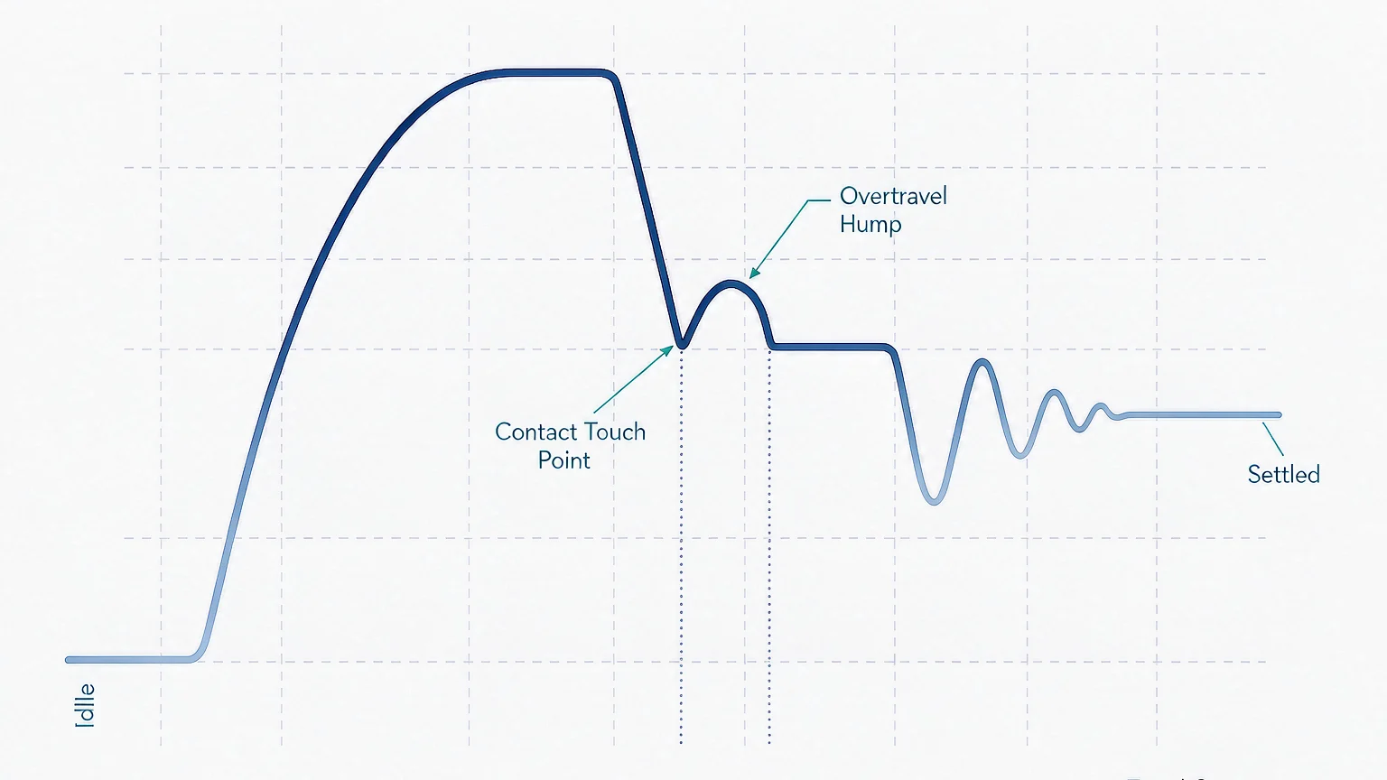
A closing operation reads left to right as a sequence of distinct phases, and each one has a different diagnostic meaning.
An opening operation has the same skeleton in reverse, with one addition: between contact separation and the extinction of the arc there is a period during which the contacts are still moving apart while current is still flowing. On a curve recorded without current, that period is invisible; it shows up as the interval between separation and the point where the travel curve reaches its final position.
A curve has hundreds of data points and six numbers that matter.
| Parameter | How it is measured | Typical HV acceptance | What it detects |
|---|---|---|---|
| Total travel | Start position to settled end position | Manufacturer value ± 2 mm | Linkage adjustment, contact wear, stop position |
| Opening velocity | Average slope over the defined arcing region | 3 – 5 m/s at 126 kV, per manufacturer | Spring energy, friction, gas pressure effect |
| Closing velocity | Average slope from command to contact touch | Lower than opening; per manufacturer | Closing spring, damper condition |
| Contact touch time | Command to main contact touch | Per manufacturer, typically 40 – 90 ms | Latch, coil, linkage, mechanism friction |
| Bounce time | First touch to final settle | ≤ 2 ms typical, ≤ 5 ms accepted | Damper, contact springs, overtravel |
| Overtravel | Peak displacement beyond touch position | Per manufacturer, typically 15 – 25 mm | Contact pressure, wear allowance |
Two more that are not on the curve but come from the same test: pole-to-pole asynchronism, typically specified at 5 ms or less on opening and 10 ms or less on closing, and coil current signature, which is recorded simultaneously and shows the armature travel and latch release as a separate waveform.
Opening velocity is not constant. It accelerates, peaks, and then decelerates into the damper. Comparing a single “maximum velocity” number between two tests is meaningless, because the peak depends on where the sample landed. The standard approach is to define an interval — usually the arcing region between contact separation and a specified point — and take the average slope over that interval. The manufacturer’s acceptance value refers to that interval, and the test must use the same one.
Most real defects produce one of five recognisable shapes.
The whole curve is stretched: longer idle time, shallower acceleration, lower velocity, longer contact touch time. The shape is preserved but the timescale is inflated. This is an energy or friction problem — a discharged or fatigued closing spring, low auxiliary supply voltage, dried-out lubrication, or a binding linkage. Check the supply voltage first, because it is free to check and it produces exactly this pattern.
The contacts reach the stop at the right speed but oscillate for 8 or 10 ms instead of 2. Velocity and travel are fine. This is a damping problem: a failed dashpot, a worn damper seal, or insufficient overtravel so the contact springs cannot absorb the kinetic energy. It is the pattern most often missed, because a technician looking at the headline velocity number sees a pass.
The curve settles, then lifts again before coming to rest. This points at the latch or the mechanical interlock rather than the contact assembly — the mechanism is not fully home and something is pushing it back. On an opening operation, a rebound suggests the latch is not engaging cleanly and the breaker may not stay open.
The contacts touch sooner and travel less than the factory curve. On an opening operation, contact separation occurs later. This is contact wear: the arcing contacts have eroded, the gap has closed up, and the mechanism is running out of stroke. The curve will show it long before the contact resistance test becomes conclusive.
Two poles match the factory curve and one does not. This is almost always a linkage, a rod end, or a per-pole adjustment rather than a mechanism problem, because the mechanism is common to all three poles. It is also the case that argues most strongly for recording all three poles on every test, not just one.
| Pattern | Curve signature | Likely cause | First check |
|---|---|---|---|
| All phases slow | Shape preserved, timescale inflated | Low energy or high friction | Auxiliary supply voltage, then spring charge |
| Long bounce | Velocity and travel normal, oscillation 8–10 ms | Damper failure or insufficient overtravel | Damper seal, dashpot oil, overtravel setting |
| Rebound after settle | Curve settles then lifts again | Latch not fully engaging | Latch and interlock, coil current signature |
| Short travel, early touch | Touch sooner, total travel reduced | Arcing contact wear | Contact resistance measurement |
| One pole differs | Two poles match factory curve, one does not | Linkage or per-pole adjustment | Rod ends, per-pole gap setting |
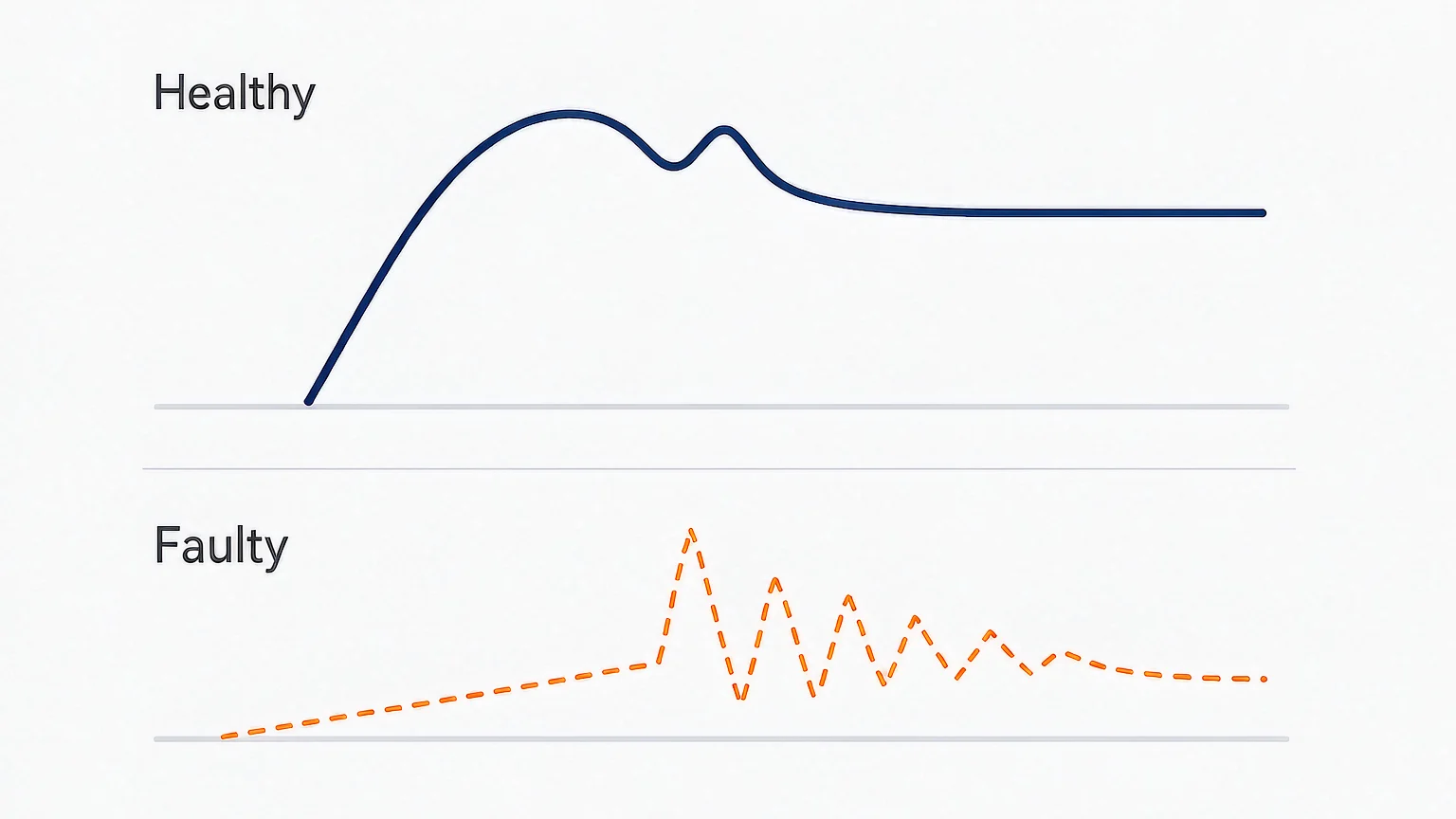
The acceptance values in the table above are orientation, not authority. The authoritative comparison is against the curve recorded at the factory, on that breaker, at commissioning, at the specified gas density and the specified ambient temperature.
That baseline is what makes the test diagnostic rather than merely pass/fail. A breaker whose opening velocity has fallen from 4.2 to 3.8 m/s over eight years is still inside a generic acceptance band, but the trend is telling you the spring is losing charge or the linkage is gaining friction, and you have several years of warning. A breaker that goes from 4.2 to 3.9 m/s in a single maintenance interval is telling you something changed suddenly.
Which is why the single most valuable thing you can do at commissioning is record the curves properly: all three poles, both operations, with the gas density, the ambient temperature and the auxiliary supply voltage written on the report. Without those four context values, a later comparison is guesswork.
It is worth being explicit about the limits, because over-reading a travel curve is as costly as ignoring it.
This is why the travel curve belongs in a test programme rather than standing alone. The SF6 circuit breaker testing guide sets out how the mechanical characteristics test sits alongside timing, contact resistance, insulation and gas tests, and what each one is for.
Four occasions, at minimum.
The maintenance planning guide covers how these intervals are set, and the failure and troubleshooting guide covers what to do when the curve shows a fault rather than a trend.
The parameters shift with the mechanism, so the acceptance values have to come from the specific product. A porcelain-column outdoor breaker with a long drive rod has more lost motion and a different velocity profile from a compact tank-type unit, and the curve reflects it.
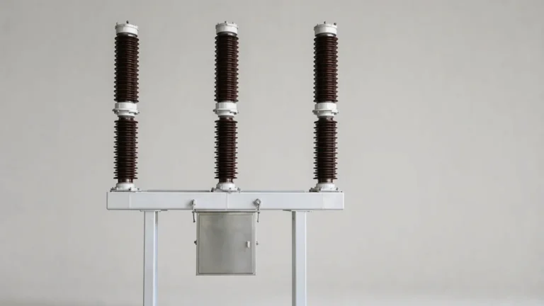
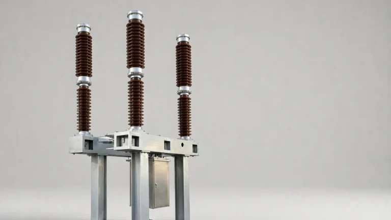
At 72.5 kV, the LW9-72.5 with 350 kV lightning impulse withstand carries a long external insulation column, and the drive train between the mechanism box and the interrupter is where most of the lost motion appears on the curve. On 40.5 kV distribution equipment, the LW8-40.5 with 3,000-operation mechanical life is designed for frequent operation, which means the cycle count — not the calendar — is what drives its wear, and the travel curve is how you confirm the wear is tracking the count. At 126 kV, the LW36-126 with 3150 A rated current uses a double-motion interrupter whose curve shows two moving contacts, so the displacement axis has to be interpreted against the relative gap rather than the travel of one rod.
The mechanism type matters too. A hydraulic drive produces a very flat velocity profile and a distinctive pressure-related tail; a spring mechanism produces a characteristic decelerating curve as the spring discharges. Reading a curve without knowing which mechanism produced it is a good way to chase a non-existent fault — the operating mechanism comparison covers the differences.
The travel curve is the highest-information, lowest-cost test available on an HV breaker. It turns a mechanism from a black box into six numbers and a shape, and the shape is specific enough to distinguish a tired spring from a failed damper from worn contacts from a loose linkage.
Record it properly at commissioning with all three poles and the context values, sample high enough to see bounce, compare against that baseline rather than a generic table, and treat a trend as seriously as a limit. Then read it alongside the gas, resistance and insulation tests rather than instead of them. For the equipment these tests apply to, the SF6 circuit breaker article library covers the rest.
A recording of contact displacement against time during an opening or closing operation, produced with a transducer on the moving contact or drive rod. It shows the idle time, acceleration, contact touch, overtravel and bounce phases of the operation.
10 kHz is enough for travel and velocity. Use 20 to 50 kHz if you are investigating bounce, because at lower rates the sample points can fall between the contact re-establishments and the bounce will not appear in the data.
Two milliseconds or less is typical for HV breakers, with up to 5 ms sometimes accepted. The more useful criterion is comparison with the factory curve: a breaker that has gone from 1.5 to 6 ms is telling you the damper has degraded regardless of what the generic limit says.
Usually low energy or high friction: a discharged closing spring, low auxiliary supply voltage, dried lubrication or a binding linkage. Check the supply voltage first because it produces the same pattern and costs nothing to verify.
Indirectly. Worn arcing contacts reduce the gap, so the contacts touch earlier and total travel falls. Confirm with a contact resistance measurement, which measures the electrical symptom directly.
Yes, every time. The mechanism is common to all poles, so a single-pole difference points at a linkage or per-pole adjustment rather than the drive — a distinction you cannot make from one trace.