Offshore Wind 66 kV Collection Systems: Breaker Selection for Salt Spray and Vibration
How 66 kV changed the collection system, what C5-M salt spray demands in measurable terms, and why the breaker boundary runs along the shoreline.
Read More
A gas-insulated switchgear bay hides every insulation defect behind earthed metal enclosures. You cannot see a discharge, smell it, or hear it from the control room — and by the time a gas quality alarm or a protection trip reveals the problem, the defect has usually been growing for months. That is exactly why partial discharge detection GIS engineers can run in service — UHF, acoustic emission and TEV sensing alongside the conventional IEC 60270 charge measurement — has become a standard acceptance and monitoring practice for SF6 circuit breakers and gas-insulated substations. This guide compares the three detection channels honestly: what each one can and cannot tell you, how sensors are placed on a real bay, which PD patterns point to which defect, and what a sensible online monitoring scope looks like for a new or retrofit substation.
Partial discharge (PD) is a localized breakdown that does not bridge the insulation gap — a spark across a void inside an epoxy spacer, a micro-discharge at a protrusion on the conductor, or a loose particle bouncing in the field. Each event is small: picocoulombs of apparent charge, nanosecond current pulses, microseconds of sound. Left alone, the same defect erodes the surrounding insulation until it fails completely.
In air-insulated substations, most PD sources announce themselves: you can hear corona, see it at night, or detect it with an ultrasonic gun from the ground. GIS removes those clues. The enclosure is a perfect Faraday cage for acoustic and visual signals, and the compact design concentrates high fields in a small volume of SF6. The consequences of missing a defect are also larger: an internal GIS fault is a bus-level event, often forcing the outage of a whole bay or busbar section while the faulted compartment is vented, cleaned and rebuilt.
Field experience across utilities consistently attributes a large share of GIS in-service failures to a handful of defect families:
| Defect type | Typical origin | Why it matters |
|---|---|---|
| Free-moving metallic particle | Assembly debris, wear from switching operations | Can migrate and bridge the gap to the enclosure; the classic GIS killer |
| Fixed protrusion on conductor or enclosure | Machining burrs, damaged finger contacts | Local field enhancement; initiates corona that erodes insulation |
| Floating electrode / loose contact | Loose shield, bolted connection that worked free | High-repetition discharges that erode contacts and generate particles |
| Void or delamination inside cast resin spacer | Casting defects, thermal cycling | Grows inside the solid insulation; invisible to gas analysis until failure |
| Surface contamination on insulator | Deposit of particles or moisture films | Tracking across the spacer surface; humidity-dependent |
Every one of these defects produces PD long before it produces a failure. The entire discipline of GIS partial discharge monitoring rests on that margin — months to years of warning, if the detection method can hear the signal.
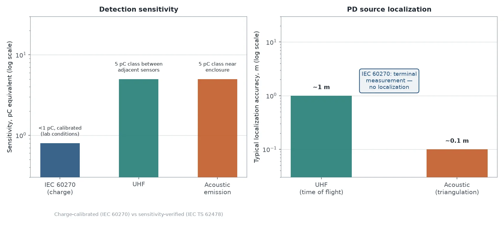
IEC 60270 is the reference method. It measures the apparent charge of each PD event in picocoulombs (pC), using a coupling capacitor and a measuring impedance at the terminals of the test object. Because the whole circuit is calibrated — a known charge pulse injected at the terminals and traced through to the instrument readout — the result is a number you can compare across tests, laboratories and manufacturers.
That calibration is the method’s strength and its constraint. The quasi-integration bandwidth is low (typically tens to hundreds of kHz), so the measurement is sensitive to interference from corona on nearby energized equipment, communication signals and switching noise. In a shielded laboratory with filtered supplies, the sensitivity is better than 1 pC. On a live substation site, the noise floor rises so far that calibrated pC measurement becomes impractical — which is why IEC 60270 work is essentially an offline, factory and commissioning-laboratory method: routine tests on individual components, type tests, and on-site commissioning measurements with the bay de-energized and excited by a resonant test set.
For buyers, IEC 60270 data matters in three places: the routine PD test certificate for each spacer and current transformer (commonly specified with limits like ≤5 pC or ≤10 pC depending on component class), the on-site AC voltage withstand plus PD measurement at commissioning, and any laboratory investigation of a suspect component. It is the yardstick every other method gets compared against — but it is not the tool you survey a live GIS hall with.
Every PD event launches a sub-nanosecond current pulse that radiates electromagnetic energy in the UHF band, roughly 300 MHz to 3 GHz. Inside a GIS the metal enclosure behaves as a waveguide: UHF pulses propagate along the compartment with attenuation of only about 0.5–2 dB per metre, reflecting off spacers and discontinuities, and leaking out at every dielectric aperture — insulator surfaces, inspection ports, bushings.
UHF sensors exploit this. A coupler detects the radiated pulse, and the instrument records amplitude, timing and phase-resolved patterns. Because the measurement band sits above most substation interference (corona and radio signals are strongest below ~300 MHz), the signal-to-noise ratio is excellent even with the bay fully energized. That is why UHF was adopted by GIS manufacturers for routine and on-site acceptance testing from the late 1980s onward, and why it remains the primary channel for continuous online monitoring.
The honest limitation: UHF does not measure charge. The received amplitude depends on the defect type, its orientation, its position and the propagation path — a “broadcast efficiency” you cannot know in advance. Converting a UHF reading in mV or dBm into picocoulombs is fundamentally not possible, so UHF readings are interpreted comparatively: against the bay’s own baseline, against trend, and against pattern signatures. The formal framework is the sensitivity check in IEC TS 62478 (electromagnetic and acoustic methods): the installed system must be able to pick up a signal equivalent to 5 pC injected between two adjacent sensors, verified with a calibrated injection — a pass/fail proof of detection capability rather than a calibrated measurement.
Sensitivity and coverage depend almost entirely on where the sensors sit:
Two or more sensors with known spacing also enable time-of-flight localization: the arrival-time difference of the same pulse (tens of nanoseconds) places the source to within roughly a metre, enough to identify the compartment before anyone plans an outage.
A discharge also injects a pressure wave into the SF6, which reaches the enclosure as structure-borne ultrasound. Piezoelectric contact sensors, magnetically or mechanically fixed to the outside of the enclosure, detect these bursts — typically in the ultrasonic band from tens to a few hundred of kHz, well above audible noise and mechanical plant vibration.
Acoustic detection has three distinctive strengths. It is almost completely immune to electromagnetic interference. It localizes precisely: an array of three or four sensors triangulates the source by arrival-time difference to within roughly 10 cm, which is the resolution you need to point at a specific spacer or contact on a opened-up inspection. And for defects close to the enclosure — free particles rolling on the floor, sparking at a floating shield — the sensitivity is very good.
Its weaknesses mirror those strengths. Attenuation through SF6 is high, so discharges deep inside the compartment (and especially inside solid spacers — voids) arrive weakly or not at all; acoustic detection misses void-type defects that UHF and IEC 60270 catch. Like UHF it cannot be charge-calibrated, and coupling quality — paint layers, rust, hand pressure on a handheld probe — directly determines what you hear. In practice acoustic emission is the confirmation and localization channel: survey the bay with UHF, then pin down the source acoustically before writing the work order.
Transient earth voltage (TEV) sensing is worth mentioning because it is often bundled into handheld survey instruments. A PD pulse reaching a discontinuity in the metal cladding — seams, gaskets, covers — produces a nanosecond voltage transient on the outer surface, picked up by a capacitive coupler in the 3–100 MHz band and reported in dBmV. TEV is the natural method for metal-clad air-insulated switchgear and ring main units, where it enables fast non-contact surveys. On welded-steel GIS the enclosure continuity limits TEV usefulness, so for gas-insulated bays it remains a secondary screen rather than a primary detector.
Gas analysis belongs to the same diagnostic family from the other direction: decomposition products such as SO2 and SOF2 accumulate as discharge energy accumulates, and SF6 decomposition products act as fault fingerprints when you need to confirm what a PD trend implies. The two views are complementary — electrical sensing finds and tracks the source, gas chemistry confirms cumulative energy and thermal involvement.
The three primary channels answer different questions, which is why serious programs run them together:
| Property | IEC 60270 (charge) | UHF | Acoustic emission |
|---|---|---|---|
| Measurand | Apparent charge (pC), calibrated | EM pulse amplitude (mV/dBm), relative | Ultrasonic burst amplitude, relative |
| Sensitivity (equivalent) | <1 pC in shielded lab | ~5 pC class between adjacent sensors (IEC TS 62478 check) | ~5 pC class near enclosure; weak for deep/void defects |
| Calibration | Full charge calibration | Not possible; sensitivity verification only | Not possible; sensitivity verification only |
| EMI immunity | Poor — needs lab conditions | Excellent — band above most interference | Excellent — acoustic domain |
| Localization | None (terminal measurement) | TOF between sensors, ~1 m class | TOF triangulation, ~10 cm class |
| Online capability | No — offline/factory method | Yes — primary continuous monitoring channel | Yes — periodic surveys and monitoring |
| Best role | Factory, type tests, commissioning acceptance | Detection, trending, PRPD classification | Confirmation and pinpoint location |
Amplitude alone never identifies a defect. The diagnostic value comes from phase-resolved PD patterns (PRPD) — plotting pulse amplitude and count rate against the 50/60 Hz cycle — combined with the pulse character on each channel:
| Defect | UHF / PRPD signature | Acoustic signature |
|---|---|---|
| Free-moving particle | Random bursts, phase-asynchronous, amplitude jumps as the particle moves | Irregular clicking or bouncing, amplitude varies with motion |
| Fixed protrusion | Symmetric clusters around voltage peaks, stable amplitude | Continuous low-level hiss |
| Floating electrode | Pulses at all phase angles, high repetition rate, often large amplitude | Strong continuous tone, sometimes audible without amplification |
| Void in spacer | Symmetric clusters just after voltage zero crossings | Usually not detectable — solid insulation shields the sound |
| Surface contamination | Low-amplitude distributed activity, grows with humidity | Weak and diffuse; cross-check with gas analysis |
Treat any pattern table as a starting hypothesis, not a verdict. The disciplined sequence is: detect and trend on UHF, classify with PRPD, localize acoustically, then confirm with gas decomposition analysis during the next planned access — the same logic used in SF6 gas quality assessment.
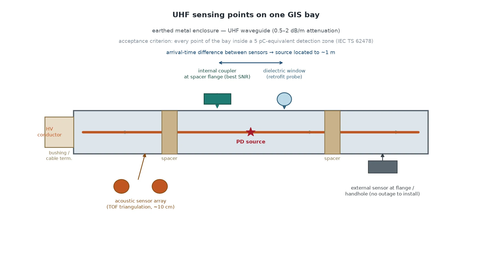
For a typical breaker-and-a-half or single-bus arrangement, sensible coverage looks like this:
The acceptance criterion for coverage is the IEC TS 62478 check between adjacent sensors — every point of the bay must be within a 5 pC-equivalent detection zone. A monitoring system that covers only half the bays is a partial answer to a whole-bay question.
A workable program usually combines three layers:
| Layer | What runs | What it catches |
|---|---|---|
| Commissioning baseline | Portable UHF + acoustic survey at energization, IEC 60270 on-site PD test where practical | Transport and assembly damage before the warranty clock starts |
| Periodic surveys | Portable UHF/AE/TEV rounds, quarterly to annually depending on criticality | Slowly developing defects; trend against baseline |
| Permanent monitoring | Fixed UHF couplers on critical bays, PRPD trending, alarm on trend | Fast-developing defects and switching-related activity between visits |
Two rules keep the data honest. First, set alarm levels from the bay’s own baseline plus margin — generic thresholds mislead because coupling, geometry and background noise differ between installations. Second, act on trend, not single readings: rising activity correlated with load or switching events justifies planning an inspection while the bay can be taken out on your schedule, not the network’s.
When GIS or its monitoring scope goes into a tender, the PD-related items worth writing down explicitly are:
The same discipline applies on the AIS side of the fence: the gas compartments of outdoor breakers are smaller but the monitoring logic is identical, and specifying a density monitor with alarm and lockout contacts is the minimum gas-side complement to any PD program. For the wider electrical environment — including the outdoor 252 kV class equipment that often surrounds a GIS hall — insulation coordination and test acceptance follow the same IEC 62271 framework described in our circuit breaker testing guide.
No single method detects everything in a GIS. IEC 60270 gives you the calibrated pC number in the factory and at commissioning; UHF gives you sensitive, interference-proof detection and trending on live equipment; acoustic emission pinpoints the source to hand-span accuracy; gas chemistry confirms what accumulated. Specified together — with sensor positions and sensitivity checks written into the purchase contract — they turn an invisible failure mode into a managed, trendable asset condition. If you are scoping PD monitoring for a new gas-insulated bay or retrofitting sensors to an existing one, our SF6 circuit breaker resource library covers the full specification chain, and our engineers can review your single-line and propose a sensing layout against it.
No. UHF amplitude depends on defect type, orientation and propagation path, so charge calibration is not physically meaningful. The standard practice is an IEC TS 62478 sensitivity check (typically a 5 pC equivalent detection requirement between adjacent sensors) plus comparative trending against the bay’s own baseline.
UHF detects the radiated bursts over the whole compartment and is the best screening channel; acoustic emission confirms and localizes the particle to within centimetres as it bounces. The combination is the fastest reliable path from “something is discharging” to “this compartment, this component”.
Yes, at the points IEC 60270 is strongest: routine certificates for components, and the on-site withstand-plus-PD acceptance test at commissioning. Continuous UHF covers the operating years; 60270 certifies the starting condition in calibrated units.
A common scheme is a baseline survey at commissioning, then quarterly to annual portable UHF/acoustic rounds depending on asset criticality, with permanent UHF monitoring reserved for critical or historically problematic bays. Alarm criteria should come from your own baseline, not generic thresholds.
Generally no — solid insulation attenuates the acoustic path severely. Void-type spacer defects are best caught by UHF patterns (clusters after voltage zero crossings) or by conventional IEC 60270 measurement on de-energized equipment.
No. PD sensing finds and tracks the active source; decomposition product analysis (SO2, SOF2, H2S) quantifies accumulated arc and discharge energy in the gas. They answer different questions, and a mature program runs both.